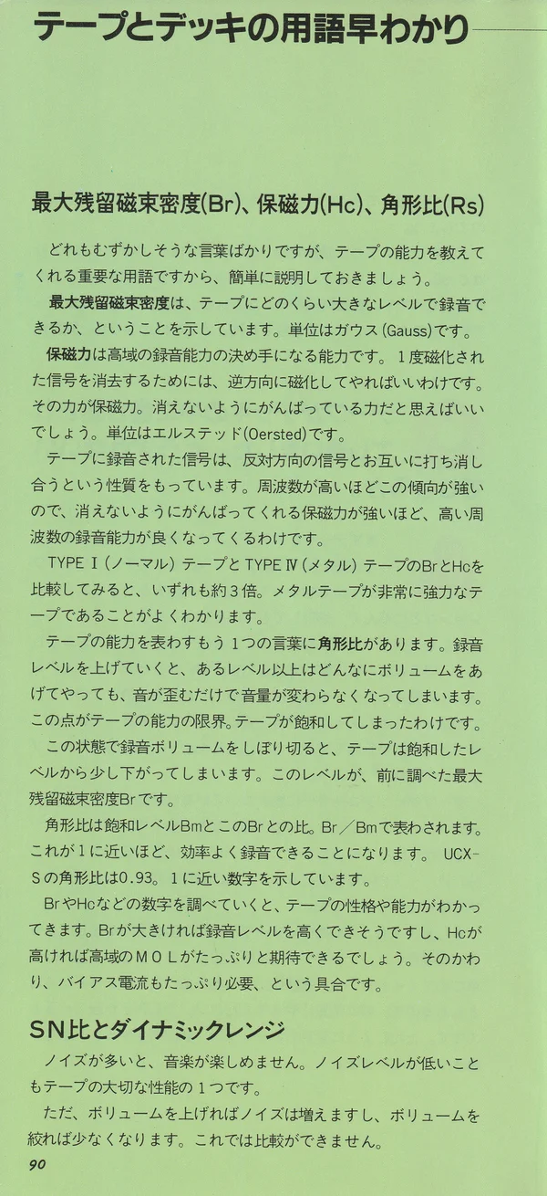
These terms all sound complicated, but they are important: they tell us what a tape can do. Let’s take a brief look at them.
Residual Magnetic Induction (Br), Coercivity (Hc) and Squareness Ratio (Rs)
Residual magnetic induction indicates how large a signal can be recorded on tape. It is measured in gauss.
Coercivity may be an unfamiliar word, but it is another important characteristic that largely determines a tape’s capabilities. To erase a previously recorded (magnetized) signal, the tape only needs to be magnetized in the opposite direction. The force that must be overcome is coercivity: you can think of it as the force with which the tape “resists” having its recording erased. It is measured in oersteds.
A signal recorded on tape has a particular property: signals in opposite directions cancel one another out. This tendency becomes stronger as frequency rises, so the greater the coercivity - the tape’s ability to “resist” erasure - the greater its high-frequency recording capability.
If you compare Br and Hc for TYPE I (Normal) and TYPE IV (Metal) tapes, both values are about three times higher on the latter. You can see just how powerful metal tape is.
Squareness ratio is another term describing a tape’s capabilities. If you increase the recording level, there comes a point where, however much more volume you add, the sound will get no louder and will only begin to distort. This is the limit of the tape’s capability: the tape has entered saturation.
If you gradually reduce the recording level, there will be a level just below the point at which the tape begins to saturate. The squareness ratio is the ratio of that level to the residual magnetic induction mentioned above.
Squareness ratio is the ratio of Br during recording to Br at saturation (Bm), expressed as Br/Bm’. The closer the value is to 1, the more efficient the recording. UCX-S has a squareness ratio of 0.93, close to 1.
Reading figures such as Br and Hc helps you understand a tape’s character and capabilities. A high Br permits a high recording level; a high Hc increases high-frequency MOL and leaves less residue after erasure. In return, more bias current is required. This is roughly how these properties are related.
Signal-to-Noise Ratio (SN) and Dynamic Range
When there is a lot of noise, you cannot enjoy music. Low noise is one of the most important tape characteristics.
But turn up the volume and the noise increases; turn it down and the noise decreases. That makes comparison impossible. Noise is most noticeable in pianissimo passages, so it makes sense to express it in relation to the music level. Yet music level is always changing and cannot be fixed as a numerical value, so a comparison with the music level is not possible either.
Instead, take as a “representative” a signal of a constant, known level that gives the same value on every measurement, and express the difference between that level and the noise level. That gives us what we need. This level is designated S, the peak S level, and because it is a ratio to noise N, it is called the “signal-to-noise ratio” (SN). S is defined as the level 0 dB above Dolby level and 4 dB above 0 VU in the EIAJ standard. Catalogs often give a figure such as 250 nW (nanowebers). At this level, even an economy TYPE I (Normal) tape can be used for enjoyable recording, so it is ideal as a “representative” of the music signal. The measurement frequency is 1 kHz; other conditions are also specified in detail.
Dynamic range, on the other hand, is needed when checking the maximum limit of what a tape can record. It is not the ratio of S to N, but the difference between the tape’s MOL and noise N. These figures can be said to show the limits of the tape’s capabilities.
Most tape noise is bias noise generated during recording, so naturally the noise will differ when the same tape is used on different decks; MOL likewise varies with the deck. Head compatibility, bias adjustment and many other conditions combine to determine the tape’s practical performance. We hope that good tape will be used on a good deck, since the deck’s own capabilities are ultimately brought out fully by the tape.
Standards and Measurement Conditions
When tape or deck specifications are published in a catalog, some basic rules or conventions are needed to compare tapes from different manufacturers.
If standards specify how measured values are expressed, they provide a guide. But measurement methods must also evolve a little for rapidly developing products such as tape recorders, or for products subject to many different rules, otherwise they cannot keep up.
Tape catalogs have included data for quite some time, so let’s gradually learn to understand it and become comfortable reading it.
In catalog data, marks such as ※ sometimes appear beside values. These indicate the measurement reference: they tell us what the data was measured against.
Let’s take a quick look at SONY cassette tape catalog data. Where ※ appears beside bias and sensitivity, the figure is the difference from a tape taken as the reference.
Maximum recording level is MOL, and here too the difference from the reference tape is shown relative to ※ 0 dB.
Another term you may be seeing for the first time is sensitivity. Sensitivity S is the difference between the maximum and minimum output levels when a low-frequency signal, such as 315 Hz, is recorded over the entire tape, expressed in dB. Naturally, the smaller this difference, the better the tape.
SOL (Saturation Output Level at high frequencies) is obtained by recording a high-frequency signal, such as 10 kHz, and measuring its output level with a VU meter.
Sensitivity data shows unevenness in the thickness of the tape’s magnetic layer, while SOL shows the smoothness of its surface. Both strongly affect sound quality. When comparing catalog data, it matters what reference was used and how the measurement was made.
DP Mechanism
Unlike an open reel, a cassette has more than half of its mechanism “hidden” in the cassette itself. The reels, tape guides and pressure pad are all closely related to how the tape behaves as it travels.
However high-performance a cassette deck may be, good results cannot be expected if the cassette shell is imprecise. This is the purpose of the cassette shell’s DP mechanism (Dual Protection Mechanism). Its main feature is a system for stable tape travel based on a combination of two-tier parallel slots.
The tape turns inside the cassette shell, so it must be held lightly from above and below with as little resistance as possible. At the same time, it must be guided evenly without damaging its edges, and measures are needed to keep the hubs from wobbling irregularly so that they rotate steadily.
For this purpose, the DP mechanism uses a parallel-slotted sheet that supports the tape at two slotted areas, ensuring stable travel. The same two areas also correct hub rotation: matching features are built into the hubs to ensure stable rotation. Combined with a precision-made shell, this sharply reduces winding problems and makes tape travel even more stable.
Wow, Flutter and Modulation Noise
These are important figures describing deck performance. Alongside wow and flutter, modulation noise has recently become a topic of discussion, so let’s see what they mean.
Wow is slow rotational speed variation. The change resembles a sound “sobbing” wow-wow, hence the imitative name “wow”. Wow is heard as a wavering sound. It is especially noticeable with a piano and similar instruments: excessive wow makes the sound undulate as if heard underwater.
Flutter is faster rotational speed variation. At rates close to wow it is heard as a fine trembling, “brrr”; at still shorter periods it is no longer perceived as wavering but appears as distortion and a clouding of the sound. The boundary between wow and flutter is 10 Hz; some standards place it at 6 Hz.
Very slow speed variation (about one cycle in several seconds) is sometimes called drift, while very fast flutter is called scrape flutter, distinguishing them in this way.
To measure wow and flutter, a correctly recorded test tape at 3,150 Hz (or 3,000 Hz) is played and its frequency measured. Without speed variation, 3,150 Hz is reproduced steadily; with variation, tape speed fluctuates and the output signal is effectively modulated. This is one way to understand wow and flutter figures. Peak is measured by the peak amplitude of the fluctuation, while RMS measures its root-mean-square value. Increasingly, W-peak is used, with measurement through a filter matched to human hearing.
Modulation noise is caused by very small variations in tape speed. When a low-frequency signal, for example several tens of Hz, is recorded, speed variations produce additional signals at various frequencies around it. Naturally, this clouds the sound. Improving the precision of the cassette shell mechanism prevents this modulation noise.
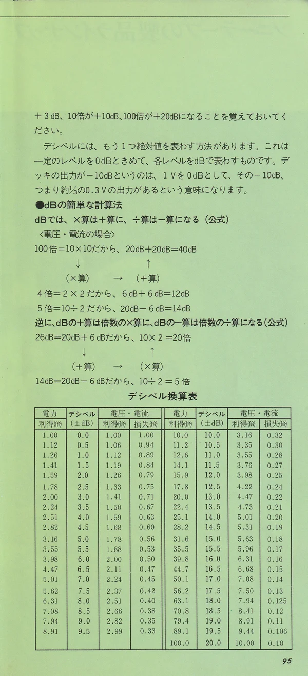
Decibel (dB)
The term “decibel” (dB) inevitably appears in tape sensitivity, frequency response, signal-to-noise ratio and similar data. It is useful to be comfortable with decibels when enjoying audio, so let’s examine them here.
The most familiar expression is something like “SN 60 dB”. SN is the ratio of signal to noise, and 60 dB represents the difference between the two levels.
The human ear perceives changes in sound not according to the difference itself, but approximately in proportion to its logarithm. Suppose the volume rises from 1 to 10. To raise it a second time and perceive the same change, adding the same difference and going from 10 to 20 is not enough. Only when it rises from 10 to 100 do we feel the same contrast as between 1 and 10.
It is therefore more convenient to use logarithms when expressing SN, sensitivity and other parameters. In dB, multiplication becomes addition and division becomes subtraction, so even signal changes spanning a very large range can easily be calculated mentally.
See the conversion table below for detailed figures. Useful approximate values to remember are: twice = +6 dB, three times = +10 dB, and ten times = +20 dB. From these it is easy to derive about 30 times = +30 dB (10 dB + 20 dB), 100 times = +40 dB (ten times is 20 dB, so 20 dB + 20 dB), and so on. It hardly needs explaining that -6 dB is about ½ and -10 dB is about ⅓.
That SN of 60 dB is 20 dB + 20 dB + 20 dB, or 10 × 10 × 10 = 1,000. The ratio of S to N is 1,000:1.
So far we have discussed voltage, current and sound pressure. For amplifier output power, however, the dB figures are halved: approximately twice is +3 dB, ten times is +10 dB, and 100 times is +20 dB. Remember this.
Decibels can also be used to express absolute values. In that case a specified level is taken as 0 dB, and other levels are expressed relative to it. If a deck’s output is -10 dB, it means 1 V is taken as 0 dB and the output is -10 dB relative to it: about ⅓, or approximately 0.3 V.
A Simple Way to Calculate in dB
In dB, multiplication becomes addition and division becomes subtraction (for voltage and current):
100 times = 10 × 10, so 20 dB + 20 dB = 40 dB
           (multiplication) → (addition)
4 times = 2 × 2, so 6 dB + 6 dB = 12 dB
5 times = 10 ÷ 2, so 20 dB - 6 dB = 14 dB
Conversely, addition in dB becomes multiplication by a factor, and subtraction becomes division:
26 dB = 20 dB + 6 dB, so 10 × 2 = 20 times
        (addition) → (multiplication)
14 dB = 20 dB - 6 dB, so 10 ÷ 2 = 5 times
Decibel Conversion Table
| Power gain (times) | ±dB | Voltage/current gain (times) | Voltage/current attenuation (times) |
|---|---|---|---|
| 1.00 | 0.0 | 1.00 | 1.00 |
| 1.12 | 0.5 | 1.06 | 0.94 |
| 1.26 | 1.0 | 1.12 | 0.89 |
| 1.41 | 1.5 | 1.19 | 0.84 |
| 1.59 | 2.0 | 1.26 | 0.79 |
| 1.78 | 2.5 | 1.33 | 0.75 |
| 2.00 | 3.0 | 1.41 | 0.71 |
| 2.24 | 3.5 | 1.50 | 0.67 |
| 2.51 | 4.0 | 1.59 | 0.63 |
| 2.82 | 4.5 | 1.68 | 0.60 |
| 3.16 | 5.0 | 1.78 | 0.56 |
| 3.55 | 5.5 | 1.88 | 0.53 |
| 3.98 | 6.0 | 2.00 | 0.50 |
| 4.47 | 6.5 | 2.11 | 0.47 |
| 5.01 | 7.0 | 2.24 | 0.45 |
| 5.62 | 7.5 | 2.37 | 0.42 |
| 6.31 | 8.0 | 2.51 | 0.40 |
| 7.08 | 8.5 | 2.66 | 0.38 |
| 7.94 | 9.0 | 2.82 | 0.35 |
| 8.91 | 9.5 | 2.99 | 0.33 |
| 10.0 | 10.0 | 3.16 | 0.32 |
| 11.2 | 10.5 | 3.35 | 0.30 |
| 12.6 | 11.0 | 3.55 | 0.28 |
| 14.1 | 11.5 | 3.76 | 0.27 |
| 15.9 | 12.0 | 3.98 | 0.25 |
| 17.8 | 12.5 | 4.22 | 0.24 |
| 20.0 | 13.0 | 4.47 | 0.22 |
| 22.4 | 13.5 | 4.73 | 0.21 |
| 25.1 | 14.0 | 5.01 | 0.20 |
| 28.2 | 14.5 | 5.31 | 0.19 |
| 31.6 | 15.0 | 5.62 | 0.18 |
| 35.5 | 15.5 | 5.96 | 0.17 |
| 39.8 | 16.0 | 6.31 | 0.16 |
| 44.7 | 16.5 | 6.68 | 0.15 |
| 50.1 | 17.0 | 7.08 | 0.14 |
| 56.2 | 17.5 | 7.50 | 0.13 |
| 63.1 | 18.0 | 7.94 | 0.125 |
| 70.8 | 18.5 | 8.41 | 0.12 |
| 79.4 | 19.0 | 8.91 | 0.11 |
| 89.1 | 19.5 | 9.44 | 0.106 |
| 100.0 | 20.0 | 10.00 | 0.10 |